Excel VBA ljestvice
Grafikoni se mogu nazvati objektima u VBA-u, slično radnom listu, također možemo umetnuti grafikone u VBA na isti način, prvo odabiremo podatke i vrstu grafikona koji želimo za vanjske podatke, sada postoje dvije različite vrste grafikona koje pružamo jedan je ugrađeni grafikon gdje se grafikon nalazi u istom listu podataka, a drugi je poznat kao list grafikona gdje se grafikon nalazi u zasebnom listu podataka.
U analizi podataka, vizualni efekti su ključni pokazatelji uspješnosti osobe koja je izvršila analizu. Vizuali su najbolji mogući način na koji analitičar može prenijeti svoju poruku. Budući da smo svi izvrsni korisnici, obično provodimo poprilično vremena analizirajući podatke i donoseći zaključke brojevima i grafikonima. Stvaranje karte je umjetnost kojom se treba ovladati i nadam se da imate dobro znanje o stvaranju karata s excelom. U ovom ćemo vam članku pokazati kako stvoriti grafikone pomoću VBA kodiranja.

Kako dodati grafikone pomoću VBA koda u Excelu?
# 1 - Stvorite grafikon pomoću VBA kodiranja
Da bismo stvorili bilo koji grafikon, trebali bismo imati neku vrstu numeričkih podataka. Za ovaj primjer koristit ću dolje opisane uzorke podataka.

Ok, prijeđimo na VBA editor.
Korak 1: Pokrenite podpostupak.
Kodirati:
Sub Charts_Example1 () Kraj Sub

Korak 2: Definirajte varijablu kao Grafikon.
Kodirati:
Sub Charts_Example1 () Zatamni MyChart kao grafikon Kraj Sub

Korak 3: Budući da je grafikon objektna varijabla, moramo ga postaviti .
Kodirati:
Sub Charts_Example1 () Dim MyChart As Chart Set MyChart = Charts.Add End Sub

Gornji kod dodati će novi list kao list grafikona, a ne kao radni list.

Korak 4: Sada moramo dizajnirati grafikon. Otvori izjavom.
Kodirati:
Sub Charts_Example1 () Dim MyChart As Chart Set MyChart = Charts.Add With MyChart End With End Sub

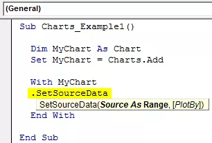
Korak 5: Prva stvar s grafikonom koju moramo učiniti je postaviti opseg izvora odabirom metode "Postavi izvorne podatke" .
Kodirati:
Sub Charts_Example1 () Dim MyChart As Chart Set MyChart = Charts.Add With MyChart .SetSourceData End With End Sub
Korak 6: Ovdje moramo spomenuti raspon izvora. U ovom slučaju, moj izvorni raspon nalazi se u listu s nazivom "Sheet1", a raspon je "A1 do B7".
Kodirati:
Sub Charts_Example1 () Dim MyChart As Chart Set MyChart = Charts.Add With MyChart .SetSourceData Sheets ("Sheet1"). Raspon ("A1: B7") End With End Sub

Korak 7: Dalje moramo odabrati vrstu grafikona koji ćemo stvoriti. Za to moramo odabrati svojstvo Vrsta grafikona .
Kodirati:
Sub Charts_Example1 () Dim MyChart As Chart Set MyChart = Charts.Add With MyChart .SetSourceData Sheets ("Sheet1"). Range ("A1: B7") .ChartType = End With End Sub
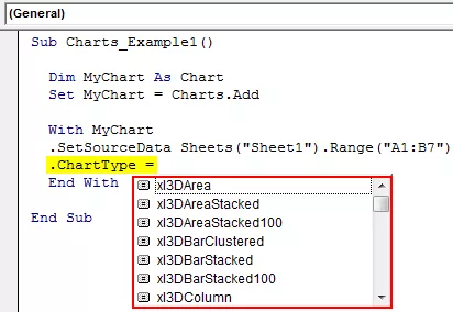
Korak 8: Ovdje imamo razne karte. Odabrat ću grafikon " xlColumnClustered ".
Kodirati:
Sub Charts_Example1 () Dim MyChart As Chart Set MyChart = Charts.Add With MyChart .SetSourceData Sheets ("Sheet1"). Range ("A1: B7") .ChartType = xlColumnClustered End With End Sub

Ok, u ovom trenutku, pokrenimo kôd pomoću tipke F5 ili ručno i pogledajte kako grafikon izgleda.

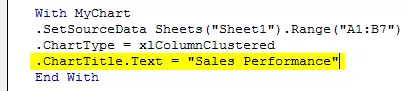
Korak 9: Sada promijenite druga svojstva grafikona. Da biste promijenili naslov grafikona, dolje je kôd.
Ovako imamo mnoštvo svojstava i metoda s grafikonima. Koristite svaku od njih da biste vidjeli utjecaj i naučili.
Sub Charts_Example1 () Dim MyChart As Chart Set MyChart = Charts.Add With MyChart .SetSourceData Sheets ("Sheet1"). Range ("A1: B7") .ChartType = xlColumnClustered .ChartTitle.Text = "End Performance" End Performance
# 2 - Stvorite grafikon s istim Excel listom kao oblik
To create the chart with the same worksheet (datasheet) as shape, we need to use a different technique.
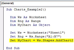
Step 1: First Declare threes Object Variables.
Code:
Sub Charts_Example2() Dim Ws As Worksheet Dim Rng As Range Dim MyChart As Object End Sub

Step 2: Then Set the Worksheet reference.
Code:
Sub Charts_Example2() Dim Ws As Worksheet Dim Rng As Range Dim MyChart As Object Set Ws = Worksheets("Sheet1") End Sub

Step 3: Now set the range object in VBA
Code:
Sub Charts_Example2() Dim Ws As Worksheet Dim Rng As Range Dim MyChart As Object Set Ws = Worksheets("Sheet1") Set Rng = Ws.Range("A1:B7") End Sub

Step 4: Now, set the chart object.
Code:
Sub Charts_Example2() Dim Ws As Worksheet Dim Rng As Range Dim MyChart As Object Set Ws = Worksheets("Sheet1") Set Rng = Ws.Range("A1:B7") Set MyChart = Ws.Shapes.AddChart2 End Sub
Step 5: Now, as usual, we can design the chart by using the “With” statement.

Code:
Sub Charts_Example2() Dim Ws As Worksheet 'To Hold Worksheet Reference Dim Rng As Range 'To Hold Range Reference in the Worksheet Dim MyChart As Object Set Ws = Worksheets("Sheet1") 'Now variable "Ws" is equal to the sheet "Sheet1" Set Rng = Ws.Range("A1:B7") 'Now variable "Rng" holds the range A1 to B7 in the sheet "Sheet1" Set MyChart = Ws.Shapes.AddChart2 'Chart will be added as Shape in the same worksheet With MyChart.Chart .SetSourceData Rng 'Since we already set the range of cells to be used for chart we have use RNG object here .ChartType = xlColumnClustered .ChartTitle.Text = "Sales Performance" End With End Sub
This will add the chart below.

#3 - Code to Loop through the Charts
Like how we look through sheets to change the name or insert values, hide & unhide them. Similarly, to loop through the charts, we need to use chart object property.
The below code will loop through all the charts in the worksheet.
Code:
Sub Chart_Loop() Dim MyChart As ChartObject For Each MyChart In ActiveSheet.ChartObjects 'Enter the code here Next MyChart End Sub
#4 - Alternative Method to Create Chart
We can use the below alternative method to create charts. We can use the Chart Object. Add method to create the chart below is the example code.
This will also create a chart like the previous method.
Code:
Sub Charts_Example3 () Dim Ws as Worksheet Dim Rng As Range Dim MyChart As ChartObject Set Ws = Worksheets ("Sheet1") Set Rng = Ws.Range ("A1: B7") Set MyChart = Ws.ChartObjects.Add (Lijevo: = ActiveCell.Left, Širina: = 400, Vrh: = ActiveCell.Top, Visina: = 200) MyChart.Chart.SetSourceData Izvor: = Rng MyChart.Chart.ChartType = xlColumnStacked MyChart.Chart.ChartTitle.Text = "Sales.Text =" Pod


